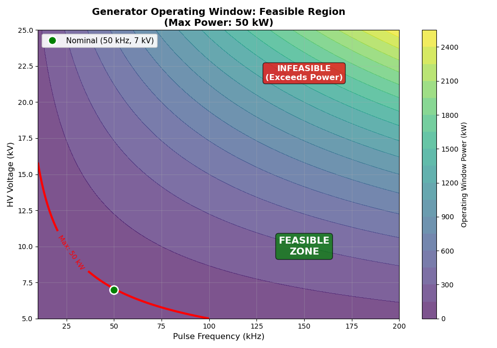
High Voltage Generator System

This example demonstrates the HighVoltageGeneratorSystem which calculates operating window constraints for the pulse power generator.

==================================================
High Voltage Generator System
==================================================
Operating Window Power: 49000.0 W
Operating Window Satisfied: Yes
==================================================
[OK] Operating point is within generator capability

Generating plot: Operating Zone (Voltage vs Frequency)...

import matplotlib.pyplot as plt
import numpy as np
import openmdao.api as om

from paroto.systems.generator import HighVoltageGeneratorSystem

# Create OpenMDAO problem
prob = om.Problem()
prob.model.add_subsystem(
    "generator",
    HighVoltageGeneratorSystem(
        design_impedance=50.0,  # 50 Ohm
        pulse_duration=1e-6,  # 1 μs
        max_power=50000.0,  # 50 kW limit
    ),
    promotes=["*"],
)
prob.setup()

# Set operating parameters
prob.set_val("pulse_frequency", 50000.0)  # 50 kHz
prob.set_val("hv_voltage", 7000.0)  # 7 kV (within feasible zone)

# Run model
prob.run_model()

# Extract results
power = prob.get_val("operating_window_power")[0]
satisfied = prob.get_val("hv_operating_window_satisfied")[0]

print("=" * 50)
print("High Voltage Generator System")
print("=" * 50)
print(f"Operating Window Power: {power:.1f} W")
print(f"Operating Window Satisfied: {'Yes' if satisfied > 0.5 else 'No'}")
print("=" * 50)

if satisfied > 0.5:
    print("[OK] Operating point is within generator capability")
else:
    print("[FAIL] Operating point exceeds generator limits")
    print("  Reduce frequency or voltage to stay within operating window")

# Plot operating zone: Voltage vs Frequency
print("\nGenerating plot: Operating Zone (Voltage vs Frequency)...")
freq_range = np.linspace(10e3, 200e3, 100)  # 10 kHz to 200 kHz
voltage_range = np.linspace(5e3, 25e3, 100)  # 5 kV to 25 kV
max_power = 50000.0  # W

# Create meshgrid
F, V = np.meshgrid(freq_range, voltage_range)

# Calculate operating window power for each (f, V) combination
# P_window = f * V^2 * t_pulse / Z
Z = 50.0  # Ohm
t_pulse = 1e-6  # s
P_window = F * V**2 * t_pulse / Z

# Create constraint satisfaction map (1 if feasible, 0 if not)
constraint_satisfied = (P_window <= max_power).astype(float)

# Create the plot
fig, ax = plt.subplots(figsize=(10, 7))

# Contour plot showing operating window power levels
contour = ax.contourf(F / 1e3, V / 1e3, P_window / 1e3, levels=20, cmap="viridis", alpha=0.7)
cbar = plt.colorbar(contour, ax=ax, label="Operating Window Power (kW)")

# Add boundary line at max power
boundary_contour = ax.contour(
    F / 1e3, V / 1e3, P_window / 1e3, levels=[max_power / 1e3], colors="red", linewidths=3
)
ax.clabel(boundary_contour, inline=True, fontsize=10, fmt="Max: %.0f kW")

# Shade the feasible region
feasible_mask = P_window <= max_power
ax.contourf(
    F / 1e3,
    V / 1e3,
    feasible_mask.astype(float),
    levels=[0.5, 1.5],
    colors=["none"],
    hatches=[""],
    alpha=0,
)

# Mark the nominal operating point
ax.plot(
    50,
    7,
    "go",
    markersize=12,
    markeredgewidth=2,
    markeredgecolor="white",
    label="Nominal (50 kHz, 7 kV)",
    zorder=10,
)

# Add labels for feasible/infeasible regions
ax.text(
    150,
    10,
    "FEASIBLE\nZONE",
    fontsize=14,
    fontweight="bold",
    color="white",
    ha="center",
    va="center",
    bbox=dict(boxstyle="round", facecolor="green", alpha=0.7),
)
ax.text(
    150,
    22,
    "INFEASIBLE\n(Exceeds Power)",
    fontsize=12,
    fontweight="bold",
    color="white",
    ha="center",
    va="center",
    bbox=dict(boxstyle="round", facecolor="red", alpha=0.7),
)

ax.set_xlabel("Pulse Frequency (kHz)", fontsize=12)
ax.set_ylabel("HV Voltage (kV)", fontsize=12)
ax.set_title(
    "Generator Operating Window: Feasible Region\n(Max Power: 50 kW)",
    fontsize=14,
    fontweight="bold",
)
ax.grid(True, alpha=0.3)
ax.legend(loc="upper left", fontsize=11, framealpha=0.9)

plt.tight_layout()
plt.show()