Torch Flow System

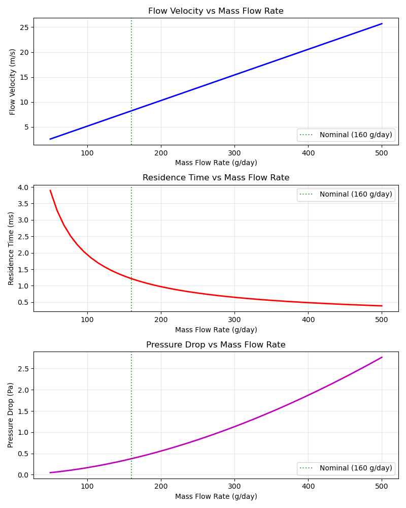
This example demonstrates the TorchFlowSystem which calculates flow velocity, residence time, and pressure drop in the plasma torch.

==================================================
Torch Flow System
==================================================
Flow Velocity: 8.22 m/s
Residence Time: 1.22 ms
Pressure Drop: 0.38 Pa
==================================================

Generating plot: Flow Characteristics vs Mass Flow Rate...

import matplotlib.pyplot as plt
import numpy as np
import openmdao.api as om

from paroto.systems.torch.flow import TorchFlowSystem

# Create OpenMDAO problem
prob = om.Problem()
prob.model.add_subsystem(
    "flow",
    TorchFlowSystem(gas_density=0.717),  # CH4 at 1 bar, 300K
    promotes=["*"],
)
prob.setup()

# Set operating parameters
prob.set_val("mass_flow", 160.0 / 86400.0)  # 160 g/day in kg/s
prob.set_val("torch_diameter", 0.02)  # 20 mm
prob.set_val("geometry_params", 0.01)  # 10 mm gap
prob.set_val("torch_length", 0.01)  # 10 mm arc length

# Run model
prob.run_model()

# Extract results
velocity = prob.get_val("flow_velocity")[0]
residence_time = prob.get_val("residence_time")[0]
pressure_drop = prob.get_val("pressure_drop")[0]

print("=" * 50)
print("Torch Flow System")
print("=" * 50)
print(f"Flow Velocity: {velocity:.2f} m/s")
print(f"Residence Time: {residence_time * 1000:.2f} ms")
print(f"Pressure Drop: {pressure_drop:.2f} Pa")
print("=" * 50)

# Plot flow characteristics vs mass flow rate
print("\nGenerating plot: Flow Characteristics vs Mass Flow Rate...")
flow_range = np.linspace(50, 500, 50) / 86400.0  # 50-500 g/day in kg/s
velocity_values = []
residence_values = []
pressure_values = []

for flow in flow_range:
    prob.set_val("mass_flow", flow)
    prob.run_model()
    velocity_values.append(prob.get_val("flow_velocity")[0])
    residence_values.append(prob.get_val("residence_time")[0] * 1000)  # ms
    pressure_values.append(prob.get_val("pressure_drop")[0])

fig, (ax1, ax2, ax3) = plt.subplots(3, 1, figsize=(8, 10))

# Plot 1: Velocity
ax1.plot(flow_range * 86400, velocity_values, "b-", linewidth=2)
ax1.axvline(x=160, color="g", linestyle=":", alpha=0.7, label="Nominal (160 g/day)")
ax1.set_xlabel("Mass Flow Rate (g/day)")
ax1.set_ylabel("Flow Velocity (m/s)")
ax1.set_title("Flow Velocity vs Mass Flow Rate")
ax1.grid(True, alpha=0.3)
ax1.legend()

# Plot 2: Residence Time
ax2.plot(flow_range * 86400, residence_values, "r-", linewidth=2)
ax2.axvline(x=160, color="g", linestyle=":", alpha=0.7, label="Nominal (160 g/day)")
ax2.set_xlabel("Mass Flow Rate (g/day)")
ax2.set_ylabel("Residence Time (ms)")
ax2.set_title("Residence Time vs Mass Flow Rate")
ax2.grid(True, alpha=0.3)
ax2.legend()

# Plot 3: Pressure Drop
ax3.plot(flow_range * 86400, pressure_values, "m-", linewidth=2)
ax3.axvline(x=160, color="g", linestyle=":", alpha=0.7, label="Nominal (160 g/day)")
ax3.set_xlabel("Mass Flow Rate (g/day)")
ax3.set_ylabel("Pressure Drop (Pa)")
ax3.set_title("Pressure Drop vs Mass Flow Rate")
ax3.grid(True, alpha=0.3)
ax3.legend()

plt.tight_layout()
plt.show()