Note
Go to the end to download the full example code.
Automatic Constraint Boundary Exploration.
Demonstrates automatic exploration of the generator operating window boundary using adaptive refinement.
This example shows how to use the constraint boundary exploration utilities to automatically find the operating limits of a high-voltage generator system without knowing the analytical constraint formula.
Setup: Import Required Modules#
Import OpenMDAO, the generator system, and the boundary exploration utilities.
import matplotlib.pyplot as plt
import numpy as np
import openmdao.api as om

from paroto.systems.generator import HighVoltageGeneratorSystem
from paroto.utils.constraint_explorer import (
    explore_constraint_boundary_2d,
    trace_constraint_boundary_2d,
)
from paroto.utils.plotting import plot_constraint_boundary, plot_operating_window
Define Generator Parameters#
Set the physical parameters for the high-voltage generator system.
# Generator operating parameters
Z = 50.0  # Design impedance (Ohm)
t_pulse = 20e-9  # Pulse duration (s) = 20 ns
P_max = 1000.0  # Maximum power (W)

print("Generator Parameters:")
print(f"  Design Impedance (Z): {Z} Ω")
print(f"  Pulse Duration: {t_pulse * 1e9:.0f} ns")
print(f"  Maximum Power: {P_max:.0f} W")
print()
Generator Parameters:
  Design Impedance (Z): 50.0 Ω
  Pulse Duration: 20 ns
  Maximum Power: 1000 W
Create OpenMDAO Problem with Generator System#
Set up a minimal OpenMDAO problem containing only the high-voltage generator system. This is the system we’ll explore.
prob = om.Problem()

# Add the high-voltage generator system
prob.model.add_subsystem(
    "generator",
    HighVoltageGeneratorSystem(
        design_impedance=Z,
        pulse_duration=t_pulse,
        max_power=P_max,
    ),
    promotes=["*"],
)

# Setup the problem
prob.setup()

# Set some nominal values (these will be overridden during exploration)
prob.set_val("pulse_frequency", 50e3)  # 50 kHz
prob.set_val("hv_voltage", 10e3)  # 10 kV

print("OpenMDAO Problem Setup Complete")
print("  Inputs: pulse_frequency, hv_voltage")
print("  Outputs: operating_window_power, hv_operating_window_satisfied")
print()
OpenMDAO Problem Setup Complete
  Inputs: pulse_frequency, hv_voltage
  Outputs: operating_window_power, hv_operating_window_satisfied
Coarse Exploration: Initial Grid Sampling#
Perform a coarse exploration of the parameter space to identify the general shape of the operating window boundary.
print("=" * 70)
print("COARSE EXPLORATION (10 × 10 grid)")
print("=" * 70)

# Define parameter ranges to explore
freq_range = (1e3, 300e3)  # 1 kHz to 300 kHz
voltage_range = (1e3, 20e3)  # 1 kV to 20 kV

# Explore with coarse grid (no refinement)
result_coarse = explore_constraint_boundary_2d(
    prob,
    param1="pulse_frequency",
    param2="hv_voltage",
    constraint_name="hv_operating_window_satisfied",
    param1_range=freq_range,
    param2_range=voltage_range,
    initial_resolution=(10, 10),
    refinement_levels=0,
    constraint_tolerance=0.2,
)

print()
======================================================================
COARSE EXPLORATION (10 × 10 grid)
======================================================================
Initial sampling: 10 × 10 = 100 points
Completed: 100 total evaluations
Found 5 points near boundary
Feasible points: 29 / 100 (29.0%)
Fine Exploration: Higher Resolution Grid#
Perform a finer exploration with higher grid resolution to get better boundary definition.
print("=" * 70)
print("FINE EXPLORATION (30 × 30 grid)")
print("=" * 70)

result_fine = explore_constraint_boundary_2d(
    prob,
    param1="pulse_frequency",
    param2="hv_voltage",
    constraint_name="hv_operating_window_satisfied",
    param1_range=freq_range,
    param2_range=voltage_range,
    initial_resolution=(30, 30),
    refinement_levels=0,
    constraint_tolerance=0.1,
)

print()
======================================================================
FINE EXPLORATION (30 × 30 grid)
======================================================================
Initial sampling: 30 × 30 = 900 points
Completed: 900 total evaluations
Found 23 points near boundary
Feasible points: 222 / 900 (24.7%)
Adaptive Refinement: Smart Exploration#
Use adaptive mesh refinement to focus evaluations near the constraint boundary. This starts with a coarse grid and automatically refines cells that contain the boundary.
print("=" * 70)
print("ADAPTIVE REFINEMENT (15 × 15 grid + 2 refinement levels)")
print("=" * 70)

result_adaptive = explore_constraint_boundary_2d(
    prob,
    param1="pulse_frequency",
    param2="hv_voltage",
    constraint_name="hv_operating_window_satisfied",
    param1_range=freq_range,
    param2_range=voltage_range,
    initial_resolution=(15, 15),
    refinement_levels=2,
    refinement_factor=2,
    constraint_tolerance=0.1,
)

print()
======================================================================
ADAPTIVE REFINEMENT (15 × 15 grid + 2 refinement levels)
======================================================================
Initial sampling: 15 × 15 = 225 points
Starting adaptive refinement: 2 level(s)
  Refinement level 1...
    Found 26 cells to refine
    Added 262 new evaluation points
  Refinement level 2...
    Found 79 cells to refine
    Added 792 new evaluation points
Completed: 1279 total evaluations
Found 418 points near boundary
Feasible points: 581 / 1279 (45.4%)
Boundary Tracing: Efficient Curve Following#
Trace the boundary curve using gradient-based continuation. This is most efficient for smooth boundaries, requiring far fewer evaluations than grid sampling.
print("=" * 70)
print("BOUNDARY TRACING (gradient-based continuation)")
print("=" * 70)

# Start from a point on the boundary
start_point = (10e3, 10000.0)  # (10 kHz, 10 kV) - should be near boundary

# Trace the boundary curve
boundary_traced = trace_constraint_boundary_2d(
    prob,
    param1="pulse_frequency",
    param2="hv_voltage",
    constraint_name="hv_operating_window_satisfied",
    start_point=start_point,
    step_size=5000.0,  # Absolute step size in parameter space
    max_points=50,
    constraint_tolerance=1e-2,
)

print()
======================================================================
BOUNDARY TRACING (gradient-based continuation)
======================================================================
Boundary tracing: Starting from (10000.0, 10000.0)
  Step size: 5000.0, Max points: 50
  Projecting start point onto boundary (initial error: 1.500000)
  Starting from: (1.224e+04, 1.426e+04)
  Traced 50 boundary points
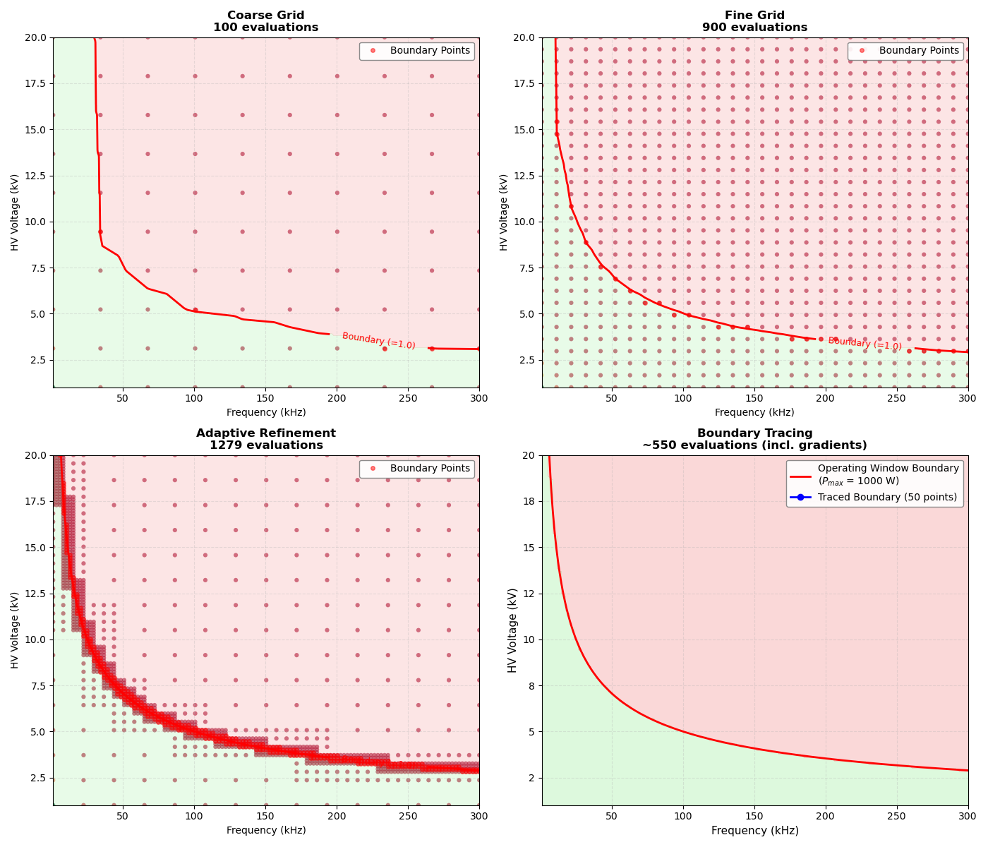
Visualization: Compare All Exploration Methods#
Create visualizations comparing: 1. Coarse exploration 2. Fine exploration 3. Adaptive refinement 4. Boundary tracing
# Helper function to convert units for display
def convert_to_display_units(result_data):
    """Convert Hz to kHz and V to kV for better readability."""
    display_data = result_data.copy()
    display_data["param1_values"] = result_data["param1_values"] / 1e3  # Hz to kHz
    display_data["param2_values"] = result_data["param2_values"] / 1e3  # V to kV
    if "boundary_points" in result_data and result_data["boundary_points"]:
        display_data["boundary_points"] = [
            (p1 / 1e3, p2 / 1e3) for p1, p2 in result_data["boundary_points"]
        ]
    return display_data


fig, axes = plt.subplots(2, 2, figsize=(14, 12))
axes = axes.flatten()

# Plot 1: Coarse Exploration
ax1 = axes[0]
result_coarse_display = convert_to_display_units(result_coarse)
plot_constraint_boundary(
    ax1,
    result_coarse_display,
    param1_name="Frequency (kHz)",
    param2_name="HV Voltage (kV)",
    show_grid_points=True,
    shade_regions=True,
    show_colorbar=False,
)
ax1.set_title(
    f"Coarse Grid\n{result_coarse['num_evaluations']} evaluations", fontsize=12, fontweight="bold"
)
ax1.legend(loc="best", framealpha=0.9, facecolor="white", edgecolor="gray")

# Plot 2: Fine Exploration
ax2 = axes[1]
result_fine_display = convert_to_display_units(result_fine)
plot_constraint_boundary(
    ax2,
    result_fine_display,
    param1_name="Frequency (kHz)",
    param2_name="HV Voltage (kV)",
    show_grid_points=True,
    shade_regions=True,
    show_colorbar=False,
)
ax2.set_title(
    f"Fine Grid\n{result_fine['num_evaluations']} evaluations", fontsize=12, fontweight="bold"
)
ax2.legend(loc="best", framealpha=0.9, facecolor="white", edgecolor="gray")

# Plot 3: Adaptive Refinement
ax3 = axes[2]
result_adaptive_display = convert_to_display_units(result_adaptive)
plot_constraint_boundary(
    ax3,
    result_adaptive_display,
    param1_name="Frequency (kHz)",
    param2_name="HV Voltage (kV)",
    show_grid_points=True,
    shade_regions=True,
    show_colorbar=False,
)
ax3.set_title(
    f"Adaptive Refinement\n{result_adaptive['num_evaluations']} evaluations",
    fontsize=12,
    fontweight="bold",
)
ax3.legend(loc="best", framealpha=0.9, facecolor="white", edgecolor="gray")

# Plot 4: Boundary Tracing
ax4 = axes[3]
# Plot analytical boundary for comparison
plot_operating_window(
    ax4,
    Z=Z,
    t_pulse=t_pulse,
    P_max=P_max,
    f_range=freq_range,
    V_range=voltage_range,
    show_annotations=False,
)
# Convert to kHz and kV for display
ax4.set_xlabel("Frequency (kHz)", fontsize=11)
ax4.set_ylabel("HV Voltage (kV)", fontsize=11)
# Update x and y tick labels
xticks = ax4.get_xticks()
ax4.set_xticklabels([f"{x / 1e3:.0f}" for x in xticks])
yticks = ax4.get_yticks()
ax4.set_yticklabels([f"{y / 1e3:.0f}" for y in yticks])
# Overlay traced boundary
ax4.plot(
    boundary_traced[:, 0] / 1e3,  # Convert to kHz
    boundary_traced[:, 1] / 1e3,  # Convert to kV
    "bo-",
    linewidth=2,
    markersize=6,
    label=f"Traced Boundary ({len(boundary_traced)} points)",
    zorder=10,
)
ax4.set_title(
    f"Boundary Tracing\n~{len(boundary_traced) * 11} evaluations (incl. gradients)",
    fontsize=12,
    fontweight="bold",
)
ax4.legend(loc="upper right", framealpha=0.9, facecolor="white", edgecolor="gray")

plt.tight_layout()
plt.savefig("generator_boundary_exploration.png", dpi=150, bbox_inches="tight")
print("Saved plot: generator_boundary_exploration.png")
/home/runner/work/paroto/paroto/examples/plot_generator_operating_window.py:286: UserWarning: set_ticklabels() should only be used with a fixed number of ticks, i.e. after set_ticks() or using a FixedLocator.
  ax4.set_xticklabels([f"{x / 1e3:.0f}" for x in xticks])
/home/runner/work/paroto/paroto/examples/plot_generator_operating_window.py:288: UserWarning: set_ticklabels() should only be used with a fixed number of ticks, i.e. after set_ticks() or using a FixedLocator.
  ax4.set_yticklabels([f"{y / 1e3:.0f}" for y in yticks])
Saved plot: generator_boundary_exploration.png
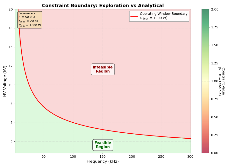
Overlay: Compare Explored vs Analytical Boundary#
Create a detailed comparison showing how well the exploration captures the analytical boundary.
fig, ax = plt.subplots(figsize=(10, 7))

# First plot the analytical boundary
plot_operating_window(
    ax,
    Z=Z,
    t_pulse=t_pulse,
    P_max=P_max,
    f_range=freq_range,
    V_range=voltage_range,
    show_annotations=True,
)

# Convert to kHz and kV for display
ax.set_xlabel("Frequency (kHz)", fontsize=12)
ax.set_ylabel("HV Voltage (kV)", fontsize=12)
# Update x and y tick labels
xticks = ax.get_xticks()
ax.set_xticklabels([f"{x / 1e3:.0f}" for x in xticks])
yticks = ax.get_yticks()
ax.set_yticklabels([f"{y / 1e3:.0f}" for y in yticks])

# Overlay the fine exploration grid points
scatter = ax.scatter(
    result_fine["param1_values"] / 1e3,  # Convert to kHz
    result_fine["param2_values"] / 1e3,  # Convert to kV
    c=result_fine["constraint_values"],
    cmap="RdYlGn",
    s=30,
    alpha=0.7,
    edgecolors="black",
    linewidth=0.5,
    vmin=0,
    vmax=2.0,
    zorder=10,
)

# Add colorbar
cbar = plt.colorbar(scatter, ax=ax)
cbar.set_label("Constraint Value\n(≥1.0 = Feasible)", rotation=270, labelpad=20)
cbar.ax.axhline(1.0, color="black", linestyle="--", linewidth=1.5)

ax.set_title("Constraint Boundary: Exploration vs Analytical", fontsize=14, weight="bold")
# Update legend with white background and transparency
legend = ax.get_legend()
if legend:
    legend.set_frame_on(True)
    legend.get_frame().set_facecolor("white")
    legend.get_frame().set_alpha(0.9)
    legend.get_frame().set_edgecolor("gray")

plt.tight_layout()
plt.savefig("generator_boundary_comparison.png", dpi=150, bbox_inches="tight")
print("Saved plot: generator_boundary_comparison.png")

plt.show()
/home/runner/work/paroto/paroto/examples/plot_generator_operating_window.py:335: UserWarning: set_ticklabels() should only be used with a fixed number of ticks, i.e. after set_ticks() or using a FixedLocator.
  ax.set_xticklabels([f"{x / 1e3:.0f}" for x in xticks])
/home/runner/work/paroto/paroto/examples/plot_generator_operating_window.py:337: UserWarning: set_ticklabels() should only be used with a fixed number of ticks, i.e. after set_ticks() or using a FixedLocator.
  ax.set_yticklabels([f"{y / 1e3:.0f}" for y in yticks])
Saved plot: generator_boundary_comparison.png
Summary and Analysis#
Compare the accuracy and efficiency of different exploration strategies.
print()
print("=" * 70)
print("SUMMARY")
print("=" * 70)
print()
print("Exploration Efficiency:")
print(f"  Coarse Grid:         {result_coarse['num_evaluations']} evaluations")
print(f"  Fine Grid:           {result_fine['num_evaluations']} evaluations")
print(f"  Adaptive Refinement: {result_adaptive['num_evaluations']} evaluations")
print(f"  Boundary Tracing:    ~{len(boundary_traced) * 11} evaluations (incl. gradients)")
print()
print("Feasible Region Coverage:")
coarse_feasible_pct = (
    100 * np.sum(result_coarse["feasible_mask"]) / result_coarse["num_evaluations"]
)
fine_feasible_pct = 100 * np.sum(result_fine["feasible_mask"]) / result_fine["num_evaluations"]
adaptive_feasible_pct = (
    100 * np.sum(result_adaptive["feasible_mask"]) / result_adaptive["num_evaluations"]
)
print(f"  Coarse Grid:         {coarse_feasible_pct:.1f}% feasible")
print(f"  Fine Grid:           {fine_feasible_pct:.1f}% feasible")
print(f"  Adaptive Refinement: {adaptive_feasible_pct:.1f}% feasible")
print()
print("Boundary Detection:")
print(f"  Coarse Grid:         {len(result_coarse['boundary_points'])} points near boundary")
print(f"  Fine Grid:           {len(result_fine['boundary_points'])} points near boundary")
print(f"  Adaptive Refinement: {len(result_adaptive['boundary_points'])} points near boundary")
print(f"  Boundary Tracing:    {len(boundary_traced)} points along boundary")
print()
print("Key Insights:")
print("  - Coarse grid (~100 pts): Quick overview of operating window")
print("  - Fine grid (~900 pts): Better boundary definition, but expensive")
print("  - Adaptive refinement: Smart compromise - refines only near boundary")
print("  - Boundary tracing: Most efficient for smooth boundaries")
print("  - All methods work for ANY constraint, not just analytical ones")
print()
print("When to Use Each Method:")
print("  - Coarse/Fine Grid: First exploration, multiple constraints")
print("  - Adaptive Refinement: Best overall - automatic + efficient")
print("  - Boundary Tracing: Known smooth boundary, need accurate curve")
print()
======================================================================
SUMMARY
======================================================================

Exploration Efficiency:
  Coarse Grid:         100 evaluations
  Fine Grid:           900 evaluations
  Adaptive Refinement: 1279 evaluations
  Boundary Tracing:    ~550 evaluations (incl. gradients)

Feasible Region Coverage:
  Coarse Grid:         29.0% feasible
  Fine Grid:           24.7% feasible
  Adaptive Refinement: 45.4% feasible

Boundary Detection:
  Coarse Grid:         5 points near boundary
  Fine Grid:           23 points near boundary
  Adaptive Refinement: 418 points near boundary
  Boundary Tracing:    50 points along boundary

Key Insights:
  - Coarse grid (~100 pts): Quick overview of operating window
  - Fine grid (~900 pts): Better boundary definition, but expensive
  - Adaptive refinement: Smart compromise - refines only near boundary
  - Boundary tracing: Most efficient for smooth boundaries
  - All methods work for ANY constraint, not just analytical ones

When to Use Each Method:
  - Coarse/Fine Grid: First exploration, multiple constraints
  - Adaptive Refinement: Best overall - automatic + efficient
  - Boundary Tracing: Known smooth boundary, need accurate curve
Total running time of the script: (0 minutes 2.239 seconds)