Initial Temperature Model

This example demonstrates the PulseInitialTemperatureModel which computes initial gas temperature accounting for energy-to-temperature conversion, cylindrical thermal diffusion, and relaxation between pulses.

The model supports different heat capacity approaches via the cp_model parameter.

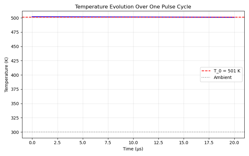
Initial Temperature T_0: 501.0 K
Peak Temperature T_max: 501.8 K
Temperature Rise ΔT: 201.8 K
Relaxation Time τ: 4929.4 μs

import matplotlib.pyplot as plt
import numpy as np
import openmdao.api as om

from paroto.models.initial_temperature import PulseInitialTemperatureModel

# Create OpenMDAO problem
# cp_model=2200 uses constant Cp (low fidelity, faster)
# cp_model=CanteraEnergyModel uses Cantera (high fidelity, requires Cantera)
prob = om.Problem()
prob.model.add_subsystem("temp", PulseInitialTemperatureModel(cp_model=2200.0))
prob.setup()

# Set parameters for typical operating conditions
prob.set_val("temp.energy_per_pulse", 10e-3)  # 10 mJ
prob.set_val("temp.pulse_frequency", 50e3)  # 50 kHz
prob.set_val("temp.thermal_diameter", 0.002)  # 2 mm arc diameter
prob.set_val("temp.arc_length", 0.01)  # 10 mm arc length
prob.set_val("temp.gas_density", 0.717)  # kg/m³ (CH4)
prob.set_val("temp.gas_heat_capacity", 2200.0)  # J/(kg·K)
prob.set_val("temp.thermal_conductivity", 0.08)  # W/(m·K)
prob.set_val("temp.ambient_temperature", 300.0)  # K
prob.set_val("temp.pulse_duration", 1e-6)  # 1 μs

# Run model
prob.run_model()

# Extract results
T_0 = prob.get_val("temp.T_0")[0]
T_max = prob.get_val("temp.T_max")[0]
delta_T = prob.get_val("temp.delta_T_pulse")[0]
tau = prob.get_val("temp.relaxation_time")[0]

print(f"Initial Temperature T_0: {T_0:.1f} K")
print(f"Peak Temperature T_max: {T_max:.1f} K")
print(f"Temperature Rise ΔT: {delta_T:.1f} K")
print(f"Relaxation Time τ: {tau * 1e6:.1f} μs")

# Plot temperature evolution over one pulse cycle
t_cycle = 1.0 / 50e3  # s
t_points = np.linspace(0, t_cycle, 100)
T_points = 300.0 + delta_T * np.exp(-t_points / tau)

plt.figure(figsize=(8, 5))
plt.plot(t_points * 1e6, T_points, "b-", linewidth=2)
plt.axhline(y=T_0, color="r", linestyle="--", label=f"T_0 = {T_0:.0f} K")
plt.axhline(y=300, color="gray", linestyle=":", label="Ambient")
plt.xlabel("Time (μs)")
plt.ylabel("Temperature (K)")
plt.title("Temperature Evolution Over One Pulse Cycle")
plt.grid(True, alpha=0.3)
plt.legend()
plt.tight_layout()
plt.show()